LaTeX tuto - Heatmaps grid with Lua

Tutorial: use Lua to automate a grid of heatmaps

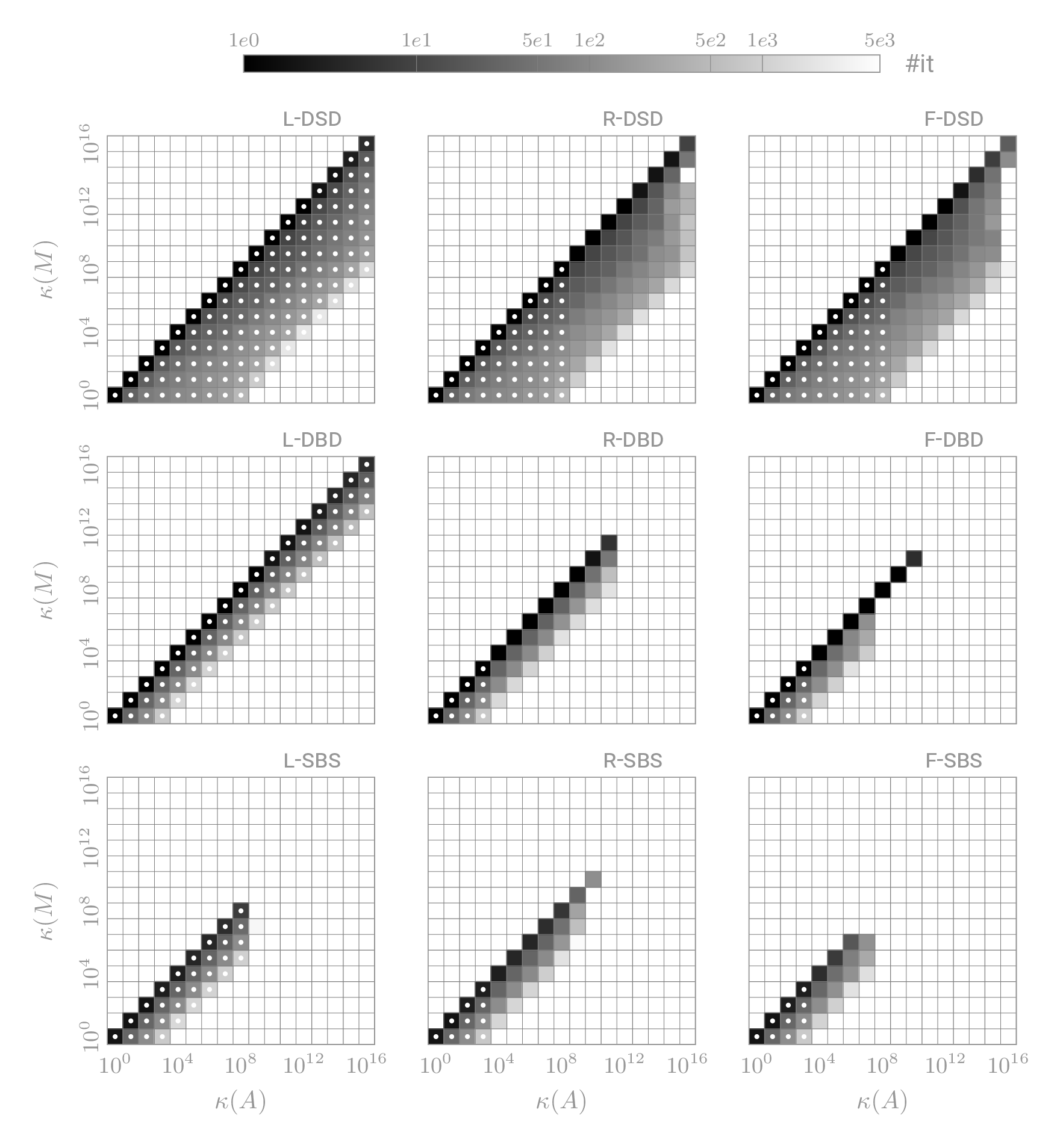
Consider the above \(3\times 3\) grid of heatmaps, where each heatmap represents the number of iterations according to \(\kappa(A)\) and \(\kappa(M)\) for a given variant of a numerical algorithm (e.g., L-DSD, F-DBD, or R-SBS). A relatively naive way to draw this plot would be to write a dedicated PGFPlots script for each of the nine heatmaps. As you can imagine, this approach has some big limitations. More specifically:

If you need to change the style of the heatmaps, you need to propagate the change nine times.
The source code will be larger and larger the bigger the number of heatmaps is.
The layout of the grid, the size of the grid, or the sources of the data cannot be changed simply.

Ultimately, we wish to write the PGFPlots script defining the style of the heatmap once and apply it nine times. Doing so, we need to take into account that from one heatmap to another there can be slight variations of style; for instance, the labels of the x- and/or y-axis may or may not be diplayed depending on the position of the heatmap in the grid. In addition, we want a convenient way to set different options for generating the grid. Specifically, we want to be able to change the grid layout (not necessarily \(3\times 3\)), the heatmaps’ size, or the sources of the data through user input parameters.

Source code for the tuto: the full compilable sources of the tuto can be downloaded from github. One can compile it at the root of the directory with

lualatex --shell-escape figure.tex

The option --shell-escape is optional and is only used to generate a .png alongside the .pdf.

Prerequisites for the tuto:

Basic notions of Lua. The Lua tutorial of tutorialspoint is a good start.
Good notions of PGFPlots, TikZ, and LaTeX. Specifically: drawing PGFPlots axis and knowing some of the basic axis options; have a basic understanding of the LaTeX macro system. One can check the PGFPlots manual if they encounter an axis option or a pgfplots command they don’t know.
Basic notions of Lua code injections in .tex document. The Alan Xiang’s Blog provides a compact and good introduction.

Origin of the figure: the figure appears in the scientific article Mixed precision strategies for preconditioned GMRES: a comprehensive analysis.

Lua automation

Achieving the above goals requires a little more than “simple LaTeX” since we need some form of automation. Notably:

Given a grid layout and the size of the heatmaps, we need to compute the position of each heatmap in the figure, accounting for the spacing between two heatmaps.
We need to compute the position and size of the colorbar.
We need to decide which heatmap will display tick labels on the x- and y-axes. In our figure, we display only x-axis labels for the heatmaps at the very bottom, and we display only the y-axis labels for the heatmaps at the very left of the grid. This allows us to save space and render a figure which is more compact and more suited for scientific journals.

This requires some scripting!

While LaTeX already offers scripting capabilities through, for instance, the LaTeX3 commands and interfaces, or other utility commands found in various libraries such as the \foreach or \pgfmathparse of the package pgfplots, the syntax is arguably less intuitive and does not match the level of tools, efficiency, and simplicity that Lua can offer.

Lua-based config file

We first tackle the problem of generating a grid of heatmaps given certain user input parameters. For this plot, we want the user to be able to set the following: the source of the data for each heatmap, the size of the heatmaps, and the number of heatmaps in one row of the grid.

Naturally, it follows the question: how does the user provide values for these parameters? As for many things in LaTeX, there is no unanimous “good answer” on how to proceed, and different approaches are valid depending on the use cases and people’s preferences. I, your tutorial master and writer of this post, have a personal preference for defining those parameters in a separate Lua config file, which is simply a Lua module that will be loaded during the compilation. This has the advantage of clearly isolating the user inputs in one dedicated place, and to not have to be stored with the rest of the LaTeX source. In this tuto, we call this file config.lua, and you can find its content below:


1
2
3
4
5
6
7
8
9
10
11
12
13
14
15
16
17
18
19
20
 -- config.lua

local config = {}

config.gridcols = 3
config.relativesize = .31
config.dircsv = "./data"
config.plots = {
  {"left_sbs", "\\textsc{l-sbs}"},
  {"right_sbs", "\\textsc{r-sbs}"},
  {"flexible_sbs", "\\textsc{f-sbs}"},
  {"left_dbd", "\\textsc{l-dbd}"},
  {"right_dbd", "\\textsc{r-dbd}"},
  {"flexible_dbd", "\\textsc{f-dbd}"},
  {"left_dsd", "\\textsc{l-dsd}"},
  {"right_dsd", "\\textsc{r-dsd}"},
  {"flexible_dsd", "\\textsc{f-dsd}"},
}

return config

In config.lua, the structure

local config = {}
  -- [...]
return config

defines a Lua module; this is simply a table of key-value referenced as config. Inside the table config, we define different keys carrying our user input parameters:

gridcols is the number of heatmaps on each row.
relativesize defines the common size of all individual heatmaps. The true size of each heatmap in the document is relativesize \(\times\) \linewidth.
dircsv sets the path to the directory containing the heatmaps’ plot data in the form of .csv files.
plots is the list of the heatmaps to be plotted. They are defined with a pair of strings. Each pair of strings is composed, first, of the name of the corresponding .csv file containing the plot data and, second, the name/title of each heatmap to be displayed in the top right corner of the plot (e.g., L-DSD, F-DBD, or R-SBS).

Our data directory dircsv looks as follows:

dircsv
├── bounds
│  ├── left_sbs.csv
│  ├── right_sbs.csv
│  └── ...
└──iterations 
    ├── left_sbs.csv
    ├── right_sbs.csv
    └── ...

The dircsv/bounds/ subdirectory contains the .csv specifying which tiles of a given heatmap have a white dot. The dircsv/iterations/ subdirectory contains the .csv that defines the number of iterations achieved on each tile.

Compute the grid layout with Lua

It is generally good practice to keep the Lua scripting out of the .tex file as much as possible. For this tutorial, we create a simple Lua module in a separate file utils.lua containing the function get_grid(...). Based on the inputs provided by the user, this function will provide three main information to the main .tex file:

The position of each heatmap in the grid.
Tell if the x- and/or y-axis labels should be displayed for a given heatmap.
The position and the size of the colorbar.

The results are passed to the .tex file through the grid object, which is a table of key-value. The full details of the utils.lua module file is displayed below.


1
2
3
4
5
6
7
8
9
10
11
12
13
14
15
16
17
18
19
20
21
22
23
24
25
26
27
28
29
30
31
32
33
34
35
36
37
38
39
40
41
42
43
44
45
46
47
48
49
50
51
52
53
54
55
56
57
58
59
60
61
62
63
64
65
66
67
68
69
70
71
72
73
74
75
76
77
78
79
80
81
 -- utils.lua

local utils = {}

function utils.get_grid(nbelt, nbcols, relativesize)

  -- Variables declaration
  local grid = {}
  local coordx, coordy = {}, {}
  local xtick, xticklabel, xlabel = {}, {}, {}
  local ytick, yticklabel, ylabel = {}, {}, {}
  local sepx   = relativesize / 5
  local sepy   = relativesize / 5
  local cbarx, cbary, cbarsizeh, cbarsizew = 0, 0, 0, 0

  -- For each heatmap, compute its position in the grid and decide to display 
  -- or not the x- and/or y-axis labels.
  for i = 1, nbelt, 1
  do
    xtick[i],  xticklabel[i], xlabel[i] = "{}", 0, "{}"
    ytick[i],  yticklabel[i], ylabel[i] = "{}", 0, "{}"
    local row = tostring(((i-1) // nbcols) * (relativesize + sepy))
    local tmp = i % nbcols
    if nbcols == 1 then
      tmp = 1
    end
    local col = tostring((tmp - 1) * (relativesize + sepx))
    if tmp == 0 then
      col = tostring((nbcols - 1) * (relativesize + sepx))
    elseif tmp == 1 then
      yticklabel[i] = 1
      ylabel[i] = "{$\\kappa(M)$}"
    end

    -- Choose the tick labels density. If the size of the heatmap is small we
    -- display less tick labels, if this is big we display more.
    if relativesize < 0.3 then
      xtick[i] = "{1,9,17}"
      ytick[i] = "{1,9,17}"
    elseif relativesize < .7 then
      xtick[i] = "{1,5,9,13,17}"
      ytick[i] = "{1,5,9,13,17}"
    elseif relativesize < 1. then
      xtick[i] = "{1,3,5,7,9,11,13,15,17}"
      ytick[i] = "{1,3,5,7,9,11,13,15,17}"
    else
      xtick[i] = "{1,2,3,4,5,6,7,8,9,10,11,12,13,14,15,16,17}"
      ytick[i] = "{1,2,3,4,5,6,7,8,9,10,11,12,13,14,15,16,17}"
    end

    coordx[i] = col .. "\\linewidth"
    coordy[i] = row .. "\\linewidth"
  end

  for i = 1, nbcols, 1
  do
    xticklabel[i] = 1
    xlabel[i] = "{$\\kappa(A)$}"
  end

  -- Compute the location and the size of the colorbar. The colorbar is located 
  -- at the top of the grid.
  cbarx = (nbcols * (relativesize + sepx) - sepx) / 2
  if (nbelt % nbcols) ~= 0 then
    cbary = (nbelt // nbcols + 1) * (relativesize + sepy) - sepy + 0.35 * relativesize
  else
    cbary = (nbelt // nbcols) * (relativesize + sepy) - sepy + 0.35 * relativesize
  end
  cbarsizew = (nbcols * (relativesize + sepx) - sepx) * 0.7
  cbarsizeh = relativesize * 0.065

  -- Put the variables in a table grid for convenience.
  grid.coordx, grid.coordy = coordx, coordy
  grid.xtick, grid.xticklabel, grid.xlabel  = xtick, xticklabel, xlabel
  grid.ytick, grid.yticklabel, grid.ylabel  = ytick, yticklabel, ylabel
  grid.cbarx, grid.cbary = cbarx, cbary
  grid.cbarsizew, grid.cbarsizeh = cbarsizew, cbarsizeh
  return grid
end

return utils

Overview of the main LuaLaTeX code

We present the main LuaLaTeX code below that will generate the grid of heatmaps. One can compile the figure with

lualatex --shell-escape heatmaps.tex

The option --shell-escape is not essential and is only used to generate a .png alongside the .pdf. The overall is embedded in a standalone LaTeX document class, which is generally the way to go to draw and generate figures outside of a main LaTeX document. Through the \includestandalone{figure} command, it is also straightforward to embed this figure into another LaTeX document (e.g., article, beamer, book, etc.).


1
2
3
4
5
6
7
8
9
10
11
12
13
14
15
16
17
18
19
20
21
22
23
24
25
26
27
28
29
30
31
32
33
34
35
36
37
38
39
40
41
42
43
44
45
46
47
48
49
50
51
52
53
54
55
56
57
58
59
60
61
62
63
64
65
66
67
68
69
70
71
72
73
74
75
76
77
78
79
80
81
82
83
84
85
86
87
88
89
90
91
92
93
94
95
96
97
98
99
100
101
102
103
104
105
106
107
108
109
110
111
112
113
114
115
116
117
118
119
120
121
122
123
124
125
126
127
128
129
130
131
132
133
134
135
136
137
138
139
140
141
142
143
144
145
146
147
148
149
150
151
152
153
154
155
156
157
158
159
160
161
162
163
164
165
166
167
168
 % figure.tex

\documentclass[convert={outext=.png},border=10pt]{standalone}
\usepackage{fontspec}
\setmainfont{Roboto}
\usepackage{pgfplots}
\pgfplotsset{compat=newest}
\usepackage{luacode}

\definecolor{fg}{RGB}{150,150,150} % Foreground color
\pgfplotsset{filter discard warning=false}

\begin{document}
%
\pgfplotsset{title style={xshift=1cm,yshift=-0.2cm}}%
%
\pgfmathdeclarefunction{lg10}{1}{ %
    \pgfmathparse{ln(#1)/ln(10)}%
}%
%
% Load utils.lua and config.lua.
\begin{luacode*}
  -- utils.lua contains lua functions to be called to be called in this file.
  myutils = require("utils")
  -- config.lua contains the user input parameters.
  myconfig = require("config")
\end{luacode*}
%
% Define a LaTeX command that generates one heatmap. Inside the command, there
% are various macros that define style options and data paths, such as,
% "\varxtick", "\varsize" or "\vardatait". These macros should be initialized 
% before calling the \heatmaps command.
\newcommand{\heatmap}
{ %
  \begin{axis}[
    % x-axis style
    minor xtick={1.5,2.5,...,16.5},
    x label style={font=\normalsize},
    xtick=\varxtick, % Recover x-ticks positions from macro
    xticklabel={
     \if\varxticklabel 1
       \pgfmathparse{\tick-1}
       $10^{\pgfmathprintnumber{\pgfmathresult}}$
     \fi
    },
    x tick label style={font=\small},
    xlabel=\varxlabel, % Recover the x-axis label from macro
    enlarge x limits={abs=0.},
    % y-axis style
    minor ytick={1.5,2.5,...,16.5},
    y label style={at={(axis description cs:-0.15,0.5)},rotate=0,font=\normalsize},
    ytick={\varytick}, % Recover y-ticks positions from macro
    yticklabel={
     \if\varyticklabel 1
       \pgfmathparse{\tick-1}
       $10^{\pgfmathprintnumber{\pgfmathresult}}$
     \fi
    },
    y tick label style={font=\small,rotate=90},
    ylabel=\varylabel, % Recover the y-axis label from macro
    enlarge y limits={abs=0.},
    % Other style
    grid=minor,
    tick style={draw=none}, % Hide the ticks
    minor grid style={fg,very thin},
    axis on top,
    mesh/ordering=y varies, 
    unbounded coords=jump,
    height=\varsize\linewidth, % Set the size (height and width) from macro
    width=\varsize\linewidth,
    colormap={whiteblue}{color={black} color=(white)},
    point meta min=0,
    point meta max=4,
    view={0}{90},
    scale only axis=true, % Enforce the paramaters height and width to describe
                          % the size of the axis without including the 
                          % decorations
    title=\textsc{\vartitle}, % Recover the name of the heatmap from macro
    at={(\varcoordx,\varcoordy)}, % Recover the position of the heatmap from
                                  % macro
  ]%
  \addplot[matrix plot*,mesh/rows=17,point meta=explicit]
      table[meta expr=lg10(\thisrow{it}),col sep=comma]
      {\vardatait}; % Obtain the data path from macro
  \addplot[white,only marks,mark=*,mark size=0.75pt] 
      table[col sep=comma] {\vardatabounds}; % Obtain the data path from macro
  \end{axis}
}%
%
% Define a LaTeX command that generates the colorbar. Because all the heatmaps
% of the grid share the same colorbar, we need to define the colorbar as a
% standalone, outside of the heatmap plots. To do so we use the 
% `\pgfplotscolorbardrawstandalone[...].`
\newcommand{\heatcolorbar}
{ %
  \pgfplotscolorbardrawstandalone[
    colormap={whiteblue}{color={black} color=(white)},
    point meta min=0,
    point meta max=3.68,
    colorbar horizontal,
    colorbar style={
       ylabel={\#it},
       yticklabel pos=upper,
       ylabel style={rotate=-90, xshift=.22cm},
       xtick={0,1,1.7,2,2.70,3,3.68},
       xticklabels={$1e0$, $1e1$, $5e1$, $1e2$, $5e2$, $1e3$, $5e3$},
       x tick label style={font=\footnotesize},
       xticklabel pos=upper,
       at={(\varcbarx\linewidth,\varcbary\linewidth)}, 
       width=\varcbarsizew\linewidth,
       anchor=center, % The position of the colorbar defined with `at` is now
       % based on the center of the figure rather than the left bottom corner
    },
    colorbar/width=\varcbarsizeh\linewidth,
    colormap access=map,
  ]%
}%
%
\begin{tikzpicture}[fg]
  \begin{luacode*}

    -- Get the grid information based on the user input parameters in
    -- config.lua and computed from the function `get_grid_heatmaps(...)`
    -- loaded from utils.lua.
    grid = myutils.get_grid(#myconfig.plots, myconfig.gridcols,
                            myconfig.relativesize)

    -- Loop over the heatmaps
    for i = 1, #myconfig.plots
    do
      
      -- Extract name of the heatmap and the source of the data from config.lua
      title   = myconfig.plots[i][2]
      pathcsv_it = myconfig.dircsv .. "/iterations/" ..  myconfig.plots[i][1] 
        .. ".csv"
      pathcsv_bounds = myconfig.dircsv .. "/bounds/" .. myconfig.plots[i][1] 
        .. ".csv"
      
      -- Set the LaTeX macros that will define the style of the current heatmap
      tex.print("\\def\\vardatait{"       .. pathcsv_it             .. "}")
      tex.print("\\def\\vardatabounds{"   .. pathcsv_bounds         .. "}")
      tex.print("\\def\\vartitle{"        .. title                  .. "}")
      tex.print("\\def\\varcoordx{"       .. grid.coordx[i]         .. "}")
      tex.print("\\def\\varcoordy{"       .. grid.coordy[i]         .. "}")
      tex.print("\\def\\varsize{"         .. myconfig.relativesize  .. "}")
      tex.print("\\def\\varxtick{"        .. grid.xtick[i]          .. "}")
      tex.print("\\def\\varxticklabel{"   .. grid.xticklabel[i]     .. "}")
      tex.print("\\def\\varxlabel{"       .. grid.xlabel[i]         .. "}")
      tex.print("\\def\\varytick{"        .. grid.ytick[i]          .. "}")
      tex.print("\\def\\varyticklabel{"   .. grid.yticklabel[i]     .. "}")
      tex.print("\\def\\varylabel{"       .. grid.ylabel[i]         .. "}")

      -- Generate the current heatmap
      tex.print("\\heatmap")
    end

    -- Set the LaTeX macros that will define the style of the colorbar
    tex.print("\\def\\varcbarx{"      .. grid.cbarx     .. "}")
    tex.print("\\def\\varcbary{"      .. grid.cbary     .. "}")
    tex.print("\\def\\varcbarsizew{"  .. grid.cbarsizew .. "}")
    tex.print("\\def\\varcbarsizeh{"  .. grid.cbarsizeh .. "}")

    -- Generate the colorbar
    tex.print("\\heatcolorbar")

  \end{luacode*}
\end{tikzpicture}%
\end{document}

Let's describe the file and its logic piece by piece, from top to bottom.

After the document class declaration, we load the different useful packages to compile the figure. The dependencies are relatively lightweight; we mostly need two main LaTeX packages (note that internally each of these two packages loads other packages):

\usepackage{pgfplots} % LaTeX package to generate a wide diversity of 
                      % scientific plots.
\usepackage{luacode}  % A set of environments and commands to ease the 
                      % Lua-LaTeX interfacing.

Once in the document’s body, we load our two Lua modules config.lua and utils.lua described in, respectively, Lua-based config file and Compute the grid layout with Lua. We load the modules as we would do it in standard Lua by writing

myutils = require("utils")
myconfig = require("config")

in a \begin{luacode*} [...] \end{luacode*} LaTeX environment, which is the environment in which Lua scripts can be executed inside a .tex document. The different functions and variables defined in the modules are now conveniently accessible through the namespaces myutils and myconfig.

We then define the “pure LaTeX” command

\newcommand{\heatmap}{
  % [...]
}

which serves to plot the heatmaps of the grid. The advantage of embedding the style of the heatmaps into one LaTeX command is that we can write the style only once and apply it multiple times.

However, as explained previously, the different heatmaps of the grid do not have exactly the same style; for example, titles, positions, or tick labels can change from one heatmap to another. A simple approach to address this issue is to pass this information as parameters of the command. For instance, by declaring the command as \newcommand{\heatmap}[2]{...}, the command \heatmap takes now two parameters. Unfortunately, a LaTeX command can only accept up to nine parameters, which cannot suit our use case here; see this StackExchange question. There are different ways to overcome this problem. We chose to rely on a LaTeX macro approach for this tutorial. With this approach, the command \heatmap is defined without parameters, but internally uses a set of LaTeX macros used as variables: \varxtick, \varxlabel, \varsize, \vardatait, etc. For instance, the macro \varsize is used to set the size of the heatmap; the macro \vardatait sets the path to the .csv file containing the data to be plotted. These macros can be redefined between each call of the command \heatmap, which allows us to change the style from heatmap to heatmap.

We define another command

\newcommand{\heatcolorbar}{
  % [...]
}

which works similarly to \heatmap. This command plots the colorbar of the figure. In more standard use cases, the colorbar is defined inside the axis environment of the plot. However, in our case, as the colorbar is shared across all the heatmaps of the grid, we use \pgfplotscolorbardrawstandalone to draw it as a standalone, which gives us more flexibility.

Finally, we enter the definition of the TikZpicture which is fully automated by Lua instructions:

\begin{tikzpicture}[fg]
  \begin{luacode*}
    % [...]
  \end{luacode*}
\end{tikzpicture}

We first call

grid = myutils.get_grid(#myconfig.plots, myconfig.gridcols, myconfig.relativesize)

which computes the grid layout based on the user input parameters of the config file. With the grid layout information computed and stored in a Lua table grid, we then loop over the heatmaps, set the variables defining the style of the current heatmap with

tex.print("\\def\\vardatait{"       .. pathcsv_it             .. "}")
tex.print("\\def\\vardatabounds{"   .. pathcsv_bounds         .. "}")
tex.print("\\def\\vartitle{"        .. title                  .. "}")
tex.print("\\def\\varcoordx{"       .. grid.coordx[i]         .. "}")
tex.print("\\def\\varcoordy{"       .. grid.coordy[i]         .. "}")
tex.print("\\def\\varsize{"         .. myconfig.relativesize  .. "}")
tex.print("\\def\\varxtick{"        .. grid.xtick[i]          .. "}")
tex.print("\\def\\varxticklabel{"   .. grid.xticklabel[i]     .. "}")
tex.print("\\def\\varxlabel{"       .. grid.xlabel[i]         .. "}")
tex.print("\\def\\varytick{"        .. grid.ytick[i]          .. "}")
tex.print("\\def\\varyticklabel{"   .. grid.yticklabel[i]     .. "}")
tex.print("\\def\\varylabel{"       .. grid.ylabel[i]         .. "}")

and generate the current heatmap by calling

tex.print("\\heatmap")

The tex.print(...) Lua function is one of the main way for Lua to provide materials to be read and interpreted by LaTeX. It basically pushes the string in parameter of tex.print in the TeX input buffer. Hence, with the previous set of Lua instructions, the LaTeX compiler will see

\def\vardatait{...}
\def\vardatabounds{...}
\def\vartitle{...}
\def\varcoordx{...}
\def\varcoordy{...}
\def\varsize{...}
\def\varxtick{...}
\def\varxticklabel{...}
\def\varxlabel{...}
\def\varytick{...}
\def\varyticklabel{...}
\def\varylabel{...}

\heatmap

At the very end, once all the heatmaps are generated, we generate the colorbar in a very similar fashion:

tex.print("\\def\\varcbarx{"      .. grid.cbarx     .. "}")
tex.print("\\def\\varcbary{"      .. grid.cbary     .. "}")
tex.print("\\def\\varcbarsizew{"  .. grid.cbarsizew .. "}")
tex.print("\\def\\varcbarsizeh{"  .. grid.cbarsizeh .. "}")

tex.print("\\heatcolorbar")

With this approach we keep as much as possible the LaTeX instructions outside of Lua scripts, and vice versa.

The overlap between LaTeX and Lua is confined to the environment

\begin{tikzpicture}[fg]
  \begin{luacode*}
    % [...]
  \end{luacode*}
\end{tikzpicture}

where we orchestrate the interactions between the user input parameters, the Lua logic, and the style of the plots expressed in LaTeX.

Examples of run

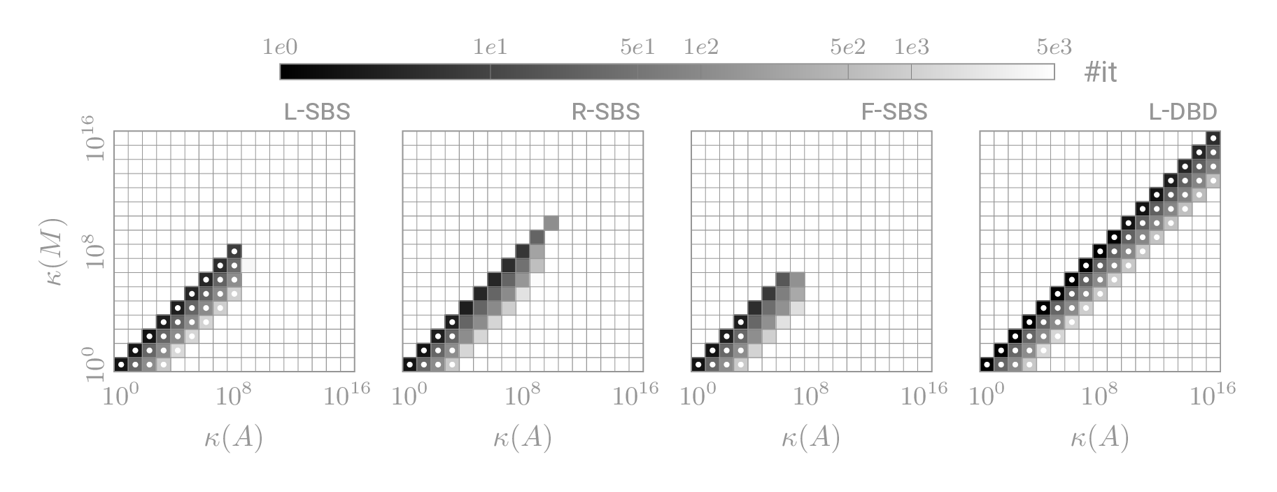
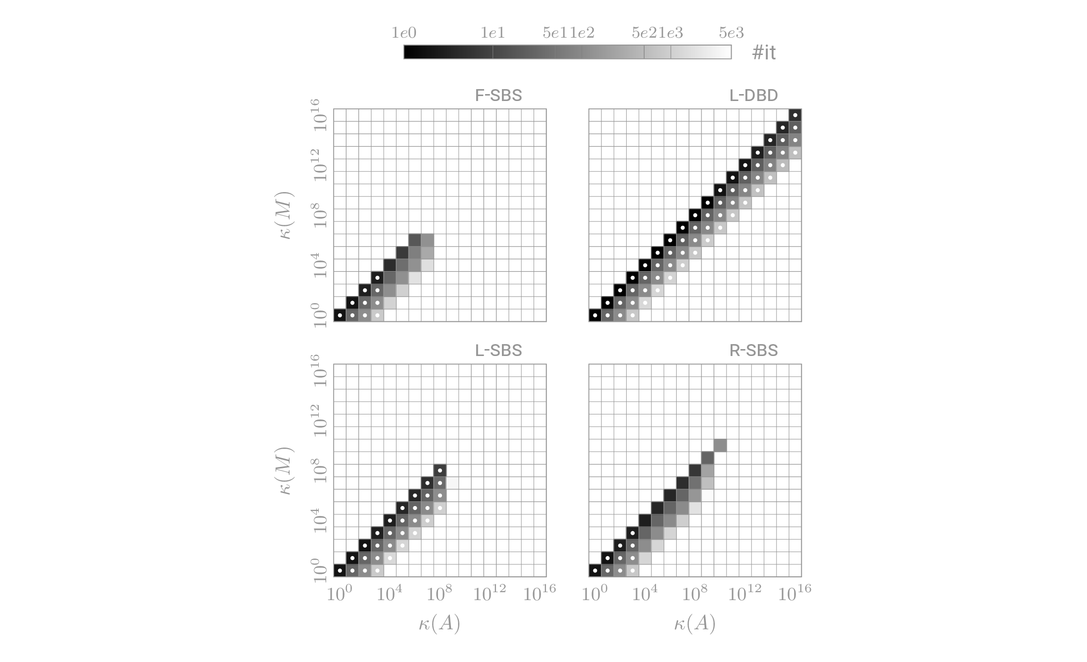
Generating different grids of heatmaps requires only changing the parameters of the config.lua file.

Example 1


1
2
3
4
5
6
7
8
9
10
11
12
13
14
15
 -- config.lua

local config = {}

config.gridcols = 4
config.relativesize = .24
config.dircsv = "./data/csv/heatmaps"
config.plots = {
  {"left_sbs", "\\textsc{l-sbs}"},
  {"right_sbs", "\\textsc{r-sbs}"},
  {"flexible_sbs", "\\textsc{f-sbs}"},
  {"left_dbd", "\\textsc{l-dbd}"},
}

return config

Example with four heatmaps in one row.

Example 2


1
2
3
4
5
6
7
8
9
10
11
12
13
14
15
 -- config.lua

local config = {}

config.gridcols = 2
config.relativesize = .3
config.dircsv = "./data/csv/heatmaps"
config.plots = {
  {"left_sbs", "\\textsc{l-sbs}"},
  {"right_sbs", "\\textsc{r-sbs}"},
  {"flexible_sbs", "\\textsc{f-sbs}"},
  {"left_dbd", "\\textsc{l-dbd}"},
}

return config

Example with a two by two grid.

Other Lua-powered figures

The same system combining Lua config file and Lua scripts with a TikZ/PGFPlots project can be used to draw many different scientific figures. Find below a few other examples: